How to turn a date into a month with Google Spreadsheets ?
Although daily events like sales or customer interactions happen on a daily basis, it's nice to get a monthly graphical perspective. In order to build those nice graphs and monthly trends, you will need to get the month from your daily dates in a nice automated way. In this article, we are exploring various ways in which you can transform your dates in month and more with Google Sheets.
1. The month() and year() functions
The month() function displays the month number from a given date, while the year() function returns the year. You can see below how this works for months (dates are in dd/mm/yyyy).

2. Combining content with the ampersand (&) character
The formula to get the year is =year(A2). If we want to combine in one single cell the year and the month, we can do this easily with the ampersand character.

Combining year(A2) and month(A2) alone works, but the result is 20121 (which is not very intuitive). To make our date clearer, we add (&) a space, dash, slash enclosed within quotation marks, eg & "-" & and the end result is 2012-1
3. Formatting the month with Text()
By default, months 1 to 9 only have one digit instead of 01 or 09. We can change this standard in two ways. With the Text function() you can help you convert a numeric/date value into text and then change the displayed format.
The Text() function only takes takes two parameters : the original value and the instruction for the new format. Formatting a month with two-digit is done with "MM". You can get a view of other formatting options on Excel Functions.net.

4. Using an IF condition to format the month
The IF condition allows you to define a value if a certain condition is met, and another value if it is not. For our date formatting exercise, we are going to add a 0 for all months with one digit, and leave the month as it is for two-digit months.
=IF(the condition;value_to_display_ if condition is met;value if condition is not met)
The simplified formula ...
=IF(month(A2)<10;"0"&month(A2);month(A2))
and the full formula with the year :
=IF(month(A2)<10;year(A2)&"-0"&month(A2);year(A2)&"-"&month(A2))

Admittedly formatting the month is much simpler with the Text() function, but we hope this practical example allowed you to discover the powerful IF() function. In the next post, we will discover various ways in which we can turn a date into a quarter.
Have fun with spreadsheets !
The IF condition allows you to define a value if a certain condition is met, and another value if it is not. For our date formatting exercise, we are going to add a 0 for all months with one digit, and leave the month as it is for two-digit months.
=IF(the condition;value_to_display_ if condition is met;value if condition is not met)
- condition : the month number if less than 10
- condition is met : add a "0" before the month(value)
- otherwise : leave the month(value) as it is
The simplified formula ...
=IF(month(A2)<10;"0"&month(A2);month(A2))
and the full formula with the year :
=IF(month(A2)<10;year(A2)&"-0"&month(A2);year(A2)&"-"&month(A2))

Admittedly formatting the month is much simpler with the Text() function, but we hope this practical example allowed you to discover the powerful IF() function. In the next post, we will discover various ways in which we can turn a date into a quarter.
Have fun with spreadsheets !

Comments
Post a Comment