How to calculate the quarter for a given date in Google Sheets
Quarterly reporting is important for many businesses. While most spreadsheets can extract the day, date, month or year from a date with dedicated functions, none of them have a built-in quarter() function. In this article we will show you how you can easily get the quarter of the year from a date.
1. The month() function
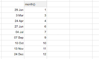
The month() function in Google Sheets gives you the month number from a date: if your cell A2 contains Sep-30 2017 or 9/30/2017, month(A2) will show "9".
2. A little math
There are four quarters in a year with three months each. Month 1 is in Q1, month 5 is in Q2, month 6 is also in Q2, while month 7 is in Q3. The logic is simple enough that we want to automate this with some math. Here is the trick : if we know the month and divide the month by 3, we are almost there :
We can see that March, June and December are in the right quarter number but for other months, the floating numbers are cause for concern. Well, not for long.
3. Rounding numbers
If we could round 0.33333333 we would certainly get our quarter. Our first shot is to use the round() function and it's a bit of failure because our numbers are rounded down by default.
4. The icing on the cake
So we have our quarter number but we really want to display "Q2". First, we are going to add some text to our cell between quotes and use a & to join to a cell or formula :
Note the ="Q"&D5 in the formula bar. That's all fine and good but it took us way too long. If we want to spare all those columns and achieve this result directly from column B, we have to combine our various formulas : ="Q"&roundup(month(A3)/3)
Happy spreading, spread the word !


Thank you.
ReplyDelete